If you are regular user of Microsoft Excel, you might aware that there are different functions in Microsoft Excel which are used for lookups viz. VLOOKUP, HLOOKUP, INDEX+MATCH etc.
In this article I’ll try to explain something exceptional in lookup functions which is easily understandable for anyone whether new to Microsoft Excel or regular user.
TWO WAY LOOKUP IN MICROSOFT EXCEL - ADVANCE EXCEL
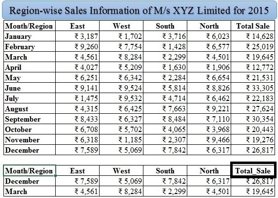
For this I have this I use, hypothetical, Region-wise Sales Information of M/s XYZ Limited for 2015 (Click here)

From this information our aim is to get all region-wise sales information for the month of March and December.
Now let see the steps.
Steps 1 Select entire table (Key board shortcut Ctrl + A)
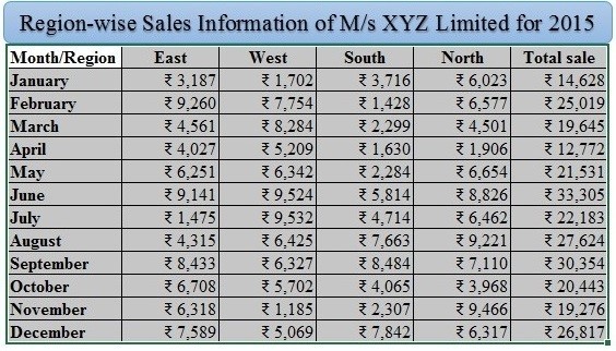
Step 2 Go to the “Create from Selection” under “FORMALAS” tab (Key board shortcut Ctrl +Shift + F3)
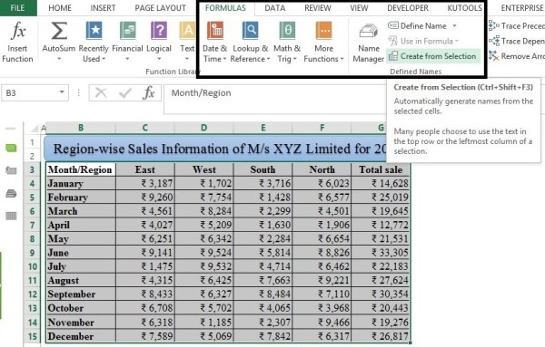
Step 3 Ensure that Top row and Left column is checked and click OK

The first three steps are just to ensure that all numeric data values have name as mentioned in their Top row and Left column. For example if you go to the name manager box (Ctrl + F3) under formula tab you will see each Microsoft Excel has defined name for all values.

For Example April has values and range.
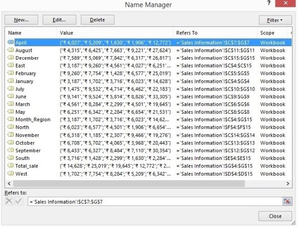
Let me explain this in much more detail, if you go the name box and select April all the data/value in front of April will get highlighted and same will also be happened for West if you select West in name box.

Step 4 Use this simple Indirect Function =INDIRECT($B18) INDIRECT(C$17) and use press Enter.

We can also use =INDIRECT(B18) INDIRECT(C17), but if we use this i.e. without putting $ sign, we will not be able to use copy + paste function accurately as range will get changed.
For example if paste this formula in D18 (December, South) it will be =INDIRECT(C18) INDIRECT(D17), Whereas we need =INDIRECT(B18) INDIRECT(D17). Same problem will also happened when we copied it to D19 (March, South)
Therefore first Indirect function we need to put $ before B column “INDIRECT($B18)”. It ensures that while using copy + paste function column will be freeze and row will be keep changing.
And for second indirect function we need to put $ sign just after “INDIRECT(C$17)” It ensures that while using copy + paste function row will be freeze and column will be keep changing.
Now all information related North, South and East gets extracted for December and March.

Note 1. for using indirect function with Name Manager we need to first ensure that reference unique column should be place at starting of the data if it is somewhere in between data i.e. we need to rearrange first.
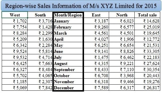
Note 2. If there is space in name, then you need to replace space with UNDERSCORE [ _ ] because while converting it into name, Microsoft Excel automatically convert these into underscores [ _ ]. For example in Total sales column there is space between Total sales and we convert it to in names Excel reads spaces as under score.

Therefore, it that cases we need to use UNDERSCORE otherwise indirect function will not work.
I hope you will be delighted with my articles, and if you have any query related to this article or anything in Microsoft Excel feel free to get in touch.
You may also make reference to my other article on Advance Excel Functions (Click here)
The author can also be reached at camukeshkumar@outlook.com


 CAclubindia
