We all are finance professionals, some may be in INDUSTRY few in PRACTICE and most of us are student to become future professionals. But whatever stage we are everyone have to face computer screen filled with Microsoft Excel Spreadsheets, outlining with financial result, budgets, forecasts and plans used to make business decisions ranging from operational to the tactical.
Most of us aware that Microsoft Excel can add, subtract, multiply and divide functions, but if we are able to use its advance functions like Vlookup, Hlookup, Index + Match etc. coupled with IF function, we can able to demeanor DATA MINING within few countable minutes which generally takes hours to complete the task and sometime impossible if we have some complex data.
Having said so, but after getting experience from different class of user of Microsoft Excel, one thing comes in mind why they people are wasting their valuable hours in completing their task in Microsoft Excel, for the things which could be completed within few minutes.
And to be honest, this gives me a sense that I should write articles as many I can on important functions Microsoft Excel.
AGEING REPORT FROM PIVOT TABLE
Excel’s Pivot Table feature is an incredibly powerful tool that makes easy to summarize data in speared sheet, particularly if someone finds difficulties in writing lots of formulas to summarize data in excel (such as COUNTIF and SUMIF). Not only to that but it also allows to quickly change how data is summarized with almost no efforts at all.
This time I will explain how to prepare a report on ageing, ageing may be for Debtor/Creditor or simple stock ageing in few seconds.
For this first you need to download practice workbook to get detailed and easy understanding of below mentioned steps. (Click Here)
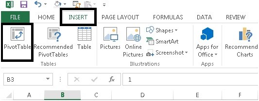
STEP-1 For creating data pivot table you need to go INSERT tab and then PIVOT TABLE.

STEP-2 The next window will be

STEP-3 In this tab you can modify range of data for Pivot table and location where pivot table. After modify, if you needed, you need to click OK

STEP-4 After this you will get this type of sheet.

STEP-5 Here you need to first drag “Product description” and “Product code” in Rows tab, “Cost” in values tab and “Holding period” in column tab.

STEP-6 After that you need to right click on holding period row and select group.

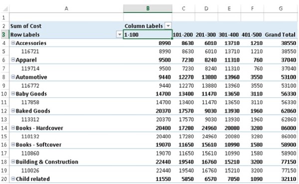
STEP-7 After selecting group you will get starting and ending numbers and range group. Here I have chosen for default "100" as range difference between lower and upper limit. You may choose something else.

STEP-8 And after your raw data is converted into meaningful report

STEP-9 But still this report need some formatting.
First select uncheck of +/- button,

STEP-10 Then go to design remove subtotal

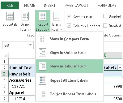
STEP-11 Select “Show in tabular form from Report layout tab

FINALLY YOUR REPORT IS READY

Hope you got an idea of this article. And if you have any query related to this article or anything in Microsoft Excel, feel free to get in touch.
The author can also be reached at camukeshkumar@outlook.com
You may also make reference on my other articles on CCI on Advance Functions of Microsoft Excel
Vlookup's Advance Function (Advance Excel)
Data Consolidation in Microsoft Excel Part-2 (Advance Excel)
Data Consolidation in Microsoft Excel (Advance Excel)
Linking Tally with Excel Steps (Advance Excel)
Scenario Manager in Excel (Revised)
Data Protection In Microsoft-Office


 CAclubindia
