" Some Economics Theories "

Others 7876 views 8 replies

Theory of Production and Cost


A firm cannot produce goods and services out of thin air. They require inputs such as land, labour (L), and capital (K). In economics, land refers to the free gifts of nature like soil, air, and water while capital refers to machines, factories and other resources. These inputs are called the

factors of production.


Production Function


The factors of production have to be combined in a particular manner to produce a certain product. Think of baking a cake which involves mixing fixed proportions of the ingredients, following a definite procedure. Indeed, baking a cake is production in economic terms. The set of all feasible combinations of factors of production and output levels produced by them is known as the production set.


The production process can be defined over 2 periods - short run and long run. In the short run, there are some factors which cannot be varied instantly. These factors are known as fixed factors. For example, labour supply depends on the population of the country which need several years to grow. Long run refers to that duration of time during which all the factors of production are variable factors.


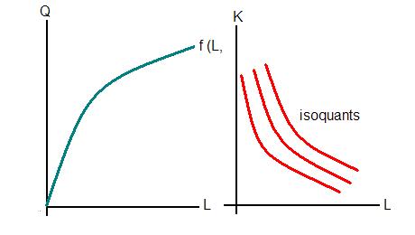
A production function expresses the maximum level of output a firm can produce using a given level of inputs. Suppose that a firm requires two inputs-capital (K) and labour (L). Its long run production function will be written as q = f (K, L). The short run production function will be q = f (L, K') where K' is the fixed input. The diagram below represents the 2 cases. Examples of production functions are the Cobb Douglas function, Leontieff technology, CES technology etc.


To go into the details of the different types of production functions avail the services provided by Transtutors.

 isoquants


Short Run Production Process


The second graph shows the output produced by varying one input alone, as happens in the short run. The blue line represents the total product generated by employing more and more labour, assuming labour is the variable factor in the 2 factor example.


Average product (AP) is the total output divided by the amount of the input used to produce this output. Mathematically, AP for labour = f (L, K') / L.


Marginal product (MP) is the change in output produced by an additional unit of an input. Mathematically, MP for labor = ? f (L, K') / ?L. Graphically, the MP is the slope of the total product curve or the production function. It indicates the rate of change in output as the input changes.

Law of Diminishing Marginal Product


This law states that given the fixed factor of production, as the amount of the variable factor is increased, a certain stage is reached beyond which the MP declines. That is, the output produced increases but at a diminishing rate. On further increasing the variable factor, the output produced starts declining.


If you are keen to know about the properties of the average and marginal products, the empirical evidence of the above mentioned law or about the general production process in the short run, come to Transtutors. Their online tutoring and assignment help can be the answer to your problems.


Long Run Production Process


The first graph depicts the long run scenario when it is possible to vary all the inputs. The red lines represent the output produced and are called isoquants. Isoquants are the locus if the feasible combinations of inputs that produce a given amount of output.


Marginal Rate of Technical Substitution (MRTS)


The MRTS of K for L is the maximum amount of L that can be replaced by one unit of K such that the level of output produced remains unchanged. It is the slope of the isoquant.


MRTS = Δf (K, L) /ΔK which is equivalent to MP of K / MP of L.

               Δf (K, L) / ΔL


Properties of isoquants:


1.      Isoquants are negatively sloped because if the quantity of factor 1 used in production is decreased then the quantity of the other factor must be increased to produce the same amount of output.


2.      Isoquants are convex to the origin. This is because of the principle of diminishing MRTS which states that as the more and more L is substituted by K, the MRTS decreases. Note that this principle is an extension of the law of diminishing MP.


3.      Higher isoquants indicate greater output yield.


4.      Isoquants do not intersect.


Elasticity of Substitution


This is measures the relative change in the input ratios in response to the change in the MRTS. It is calculated by dividing the percentage change in L/K by the percentage change in the MRTS of K for L.


Returns to Scale


The law of diminishing marginal product applies in the short run when labour is the only variable input. In the long run, a firm can change the scale of production by varying all its input. How does the output change in that case? At the beginning of the period, there occurs increasing returns to scale followed by constant returns to scale. If the inputs are increased further then there is decreasing returns observed also.


Increasing returns to scale (IRS) - This implies that if all the inputs of the firm are increased λ times then more than λ times output will be produced. Mathematically, f(λK, λL) > λf(K, L). The IRS can used in defence of mergers because one logical extension of this condition is that two identical small firms would produce more output if they were to combine their resources and become one large firm.
 

Constant returns to scale (CRS)  - If a firm increases the amount of all of its inputs λ times and output also increases λ times then the production function exhibits constant returns to scale, i.e., f(λK, λL) = λf(K, L).


Decreasing returns to scale (DRS) - When a firm increases its inputs λ times but the output produced is less than λ times then the firm is said to exhibit decreasing returns to scale. f(λK, λL) < λf(K, L).


Professional tutors at Transtutors can solve all your doubts in this topic. Choose between the online tutoring and homework help facilities provided to suit your needs.


Replies (8)

Optimum Choice of Firms


The most important decision to be taken by a firm is about the amount of output to be produced. The objective of all firms is to maximize profit. Profit is the total revenue earned by the firm minus the costs incurred during production. Given the price of the product, the revenue of the firm depends on the amount of the product produced. In order to maximize profit, a firm must minimize the costs of production given a level of output or it must maximize the output produced given the total expenditure. Therefore, the optimal choice of factor combinations depends on the technological possibilities of production, which we have examined in the previous sections, and the prices of factors.


Prices of factors used


The cost of capital if called rent in economics while labourers need to be paid wages. Suppose that the rent is $r and wage is $w per day. The total cost to the firm will be


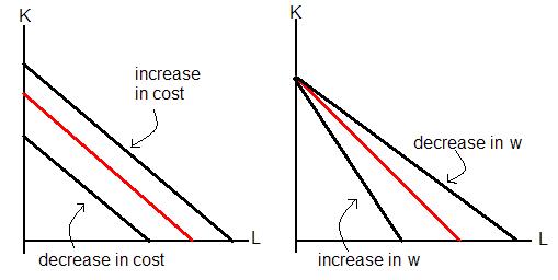
C = rK + wL where K and L are the quantities of capital and labour employed in the process. For any given value of C, the equation can be plotted on a graph as a straight line with absolute slope equal to w/r. This line is called an isocost line and is the locus of factor combinations which can be purchased for a particular total cost. The first graph shows how the red isocost line will shift with changes in the total cost outlay. The isocost line will tilt inward or outward depending on the increase or decrease in the factor costs as illustrated in graph 2.


increase-in-cost


Optimum Factor Combination


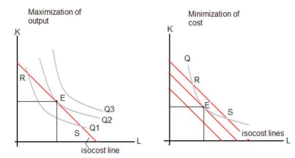
To locate the point on the graph at which production should take place so as to maximize profit, the following condition must be satisfied. At the optimal point (E), slope of the isoquant = slope of the isocost line which is equivalent to MRTS = MPK / MPL = w / r.


This will hold whether the firm attempts to maximize output subject to the cost constraint or minimize costs given the output level.


Careful notice the diagram below to understand how to solve the firm's problem graphically. At R and S, the input combinations required either do not produce the maximum possible output or are too costly for the firm. The solution, therefore, is E.

maximization-of-output


Finding the optimal factor combination graphically can be tiresome and not effective if there are more than 2 inputs involved. It then becomes necessary to use mathematics. The firm has to solve the constrained output maximization problem or the constrained cost minimization problem. Using the Langrangian method we can also arrive at the solution mathematically. The solution will give us the amounts of input demanded by the firm to produce the optimal amount of output. The input combinations that solve the maximization problem are known as the demand function. The input amounts will be functions of the input and the product prices. On the other hand, the solution to the minimization problem are called the derived or conditional factor demand function and are dependent on the factor prices as well as the specified output level.


In the short run, output produced depends on the amounts variable factor employed. Then the condition for profit maximization becomes: MPL = w/p, assuming labor is the variable factor and p is the price of the product.


The most important thing to learn here is the Lagrangian method of optimization. Ensure you master this method with the help of online tutoring session at Transtutors. Then it will be easy to deal with the multiple factors case.


Comparative Statics


Inverse Demand Function


If variable factor prices changes, then the isocost line will tilt and consequently, the optimal factor requirement will be different. Suppose the wage rate of labor is allowed to vary. The resulting locus of profit maximizing amount of labor is referred to as the inverse demand function for labor. It measures what the price of labor must be to get certain units of labor, when the level of the other factor is fixed.

inverse-demand-function


Expansion Path


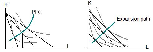
This line shows how the factor combinations utilized by a firm changes as it expands its level of output. It is the locus of points of tangency between the isoquants and isocost lines.


Price Factor Curve (PFC)


Holding total cost fixed, factor prices are allowed to vary. If e change the price of L and hold the price of K fixed then the isocost will tilt. The locus of optimal factor combination points is known as the price factor cost. Note that this is the long run equivalent of the inverse demand function.


PFC(Price Factor Curve )


Effect of Change in the Factor Price


The total effect of a change in the price of a factor can be divided in 2 - the expansion or output effect and the technical substitution effect. The output effect refers to the changes caused due to the alterations in the total cost. Technical substitution effect is the result of the change in the relative price of the factors. This is similar to the effect of changes in the price of a commodity that we mentioned under Slutsky equation.


Expenditure Elasticity


This measures the percentage change in the factor used in response to the change in the total cost. If this value is greater than 0 then the factor is superior, otherwise it is inferior.


When it comes to application of the theory of production, comparative statics is widely utilized. To gain more knowledge in this topic, take the assistance of online tutoring and assignment help at Transtutors.


Costs


If raw materials, machines and other things required for production could be made available freely then the study of the theory of the production and indeed, the study of economics would be useless! However, a firm has to incur costs of all kinds which demand serious attention.


Cost Function


A cost function expresses the relation between total cost and the cost minimizing level of output. Mathematically, C = C(y) where y is the optimal output level.


Short Run


In the short run there are 2 kinds of costs - fixed costs and variable costs. Fixed costs are the costs of the fixed factors and do not change with the changes in the level of output produced. Variable costs, which are the cost of the variable factors, change with the change in the production level.


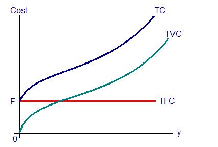
C(y) = TC = TFC + TVC, where TC is total cost, TFC is total fixed cost and TVC is total variable cost.


If K and L are the fixed and variable factors respectively, whose prices are r and w then

TC = wL + rK.


Since L depends on the output produced,


TC = wL(y) + F where F is a constant.


short-run


In the above graph note the following features:


  1. When y = 0, TFC = F, TVC = 0, TC = F.
  2. The vertical distance between TC and TVC remains constant and is equal to F.
  3. As y rises, TVC increases and so does TC.


Average Fixed Cost (AFC)


AFC is the fixed cost per unit of output.


AFC = TFC/y


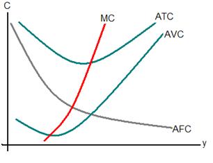
Since the TFC is constant throughout the short run, as y increases AFC will decline. Therefore, the AFC curve is downward sloping.


Average Variable Cost (AVC)


AVC is the variable cost per unit of output.


AVC = TVC/y.


AVC will generally decrease as the output increases. But because of the operation of the law of diminishing marginal product, the AVC will rise after a certain point. Notice that is it a mirror image of the average product curve. Manipulating the formulae of both will prove that AVC is inversely related to AP.


Average Total Cost (ATC)


ATC is the total cost per unit of output.


ATC = TC/y = (TFC + TVC)/y = AFC +AVC


ATC falls sharply at the beginning of the production process because both AVC and AFC are declining. When AVC begins rising but AFC is falling steeply, then the ATC continues to fall. Then the AVC rises sharply and offsets the fall in AFC causing the ATC to fall. The shape of the ATC curve is almost u-shaped.


Marginal Cost (MC)


MC is the addition to the total cost generated by increasing production by one unit. It is the slope of the TC curve. Mathematically, MC = ?TC / ?y.


The behaviour of the marginal product curve determines the MC curve, which is the inverse of the former.


Before to attempt to plot the cost curves, it is important to know the rules of averages and marginal quantities. According to these mathematical rules,


When MC < AC then AC decreases.


When MC > AC then AC rises.


When MC = AC then average costs are at the minimum.


short-run


Long Run


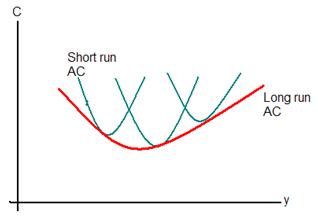
In the short run, the size of the plant is fixed whereas in the long run a firm can adjust its plant size. One of the choices in the long run will be the short run plant size. That is, a particular level of output will be the optimum choice in both periods. So, short run average cost curves must be tangent to the long run average cost curve. A long run involves several short runs. Consequently, the long run average cost curve will be the lower envelope of the short run cost curves.


long-run


The firm chooses that amount of fixed factors to minimize the average costs. In the long run marginal cost curves will consist of different parts of the short run marginal cost curves for each level of the fixed factor. The long run MC will be u-shaped and will intersect the long run average curve at the minimum.


No analysis of a firm can be complete without the analysis of its cost structure. Transtutors provides services like online tutoring and assignment help where you can learn about the details of short run as well as the long run cost functions.


Theory of Consumer Behavior


A consumer is a unit of consumption and one of the agents in the commodity market. A consumer has a certain amount of income he can use to buy goods and services from the market. Given the fixed income and fixed prices of the goods, the consumer has to decide whether to buy a particular good and what amount of it to buy. So, the consumer faces the problem of choice of commodity. This problem can be solved on the basis of the economic theory of consumer behavior - consumers choose the best bundle of goods they can afford. Therefore, the problem can be viewed from 2 sides - affordability and preference.


Affordability


Each consumer would like to buy endless number of commodities that are available in the market. However, the number of commodities a consumer can afford depends on the prices of the different commodities and the income of the consumer. This limit to what the consumer can afford to buy is what we call the budget constraint.


Let us consider a situation where there are n numbers of commodities available to a consumer. We also suppose that the price of these commodities in the market are (p1, p2, ...., pn) and the income of the consumer is m. The budget constraint can then be written as


                                          p1x1+p2x2+.....+pnxn ≤ m


where (x1, x2,....., xn) represent the amounts of the different commodities bought. This vector is the budget set of the consumer at (p1, p2, ...., pn) prices and m income.


The budget constraint, therefore, specifies that the total amount of money spent on the different commodities cannot exceed income of the consumer.


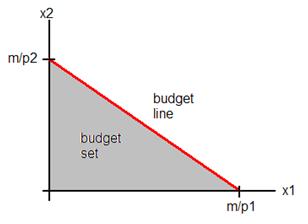
If we assume that there are only 2 goods (x1 and x2) in the market then we can represent the budget set on a graph.


budget-line


The budget line is the vector of those commodities whose cost is equal to m. The bold red line in the diagram is the budget line while the grey area represents the budget set.


From the diagram we can observe a few nice properties of the budget set:

  1. The budget set is bounded from all sides by the positive axes and the budget line. This implies that a consumer cannot buy negative amounts of either commodity.
  2. The set is closed since the consumer cannot spend more than his income.
  3. The slope of the budget line is - p1/ p2. If the consumer wishes to consume more of one commodity then he has to consume less of the other. The slope is sometimes referred to as the opportunity cost of commodity 1.


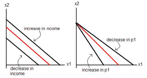
The budget constraint of an individual is not the same forever. If the prices of the commodities or the income of the consumer changes then the number of commodities and the amounts that can be bought also increases or decreases.


If the income, m increases then more commodities can be bought. This is depicted by an outward shift of the budget line. A decrease in the prices by an equal amount will have a similar effect. If the price of any one good increases, then the budget line will tilt inwards narrowing down the budget set of the consumer. However, if the income and the prices rise at an equal rate then budget line and hence, the budget set will remain the same.


budget-constraints


Budget constraint is a very important concept in economics and is utilized even in advanced economic theory. Let the competent tutors at Transtutors guide you in understanding the concept thoroughly. Try the online tutoring and homework help provided by them.


Preference


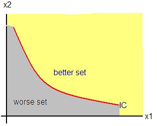
Suppose there are 2 commodity bundles - x' and x'. Each bundle has certain amount of the 2 goods x1 and x2. There are 3 ways of expressing the preference of an individual over x' and x'.


(i)                 Consumer strictly prefers x' to x'. Given the option, he would choose x' over x'. x' is said to belong to the better set of x'.

(ii)               Consumer strictly prefers x' to x'. Then x' belongs to the worse set of x'.

(iii)             Consumer is indifferent between x' and x', i.e., he would be equally satisfied with x' as with x'. The 2 bundles then belong to the same indifference set.


In economics, consumers are assumed to be rational individuals. Consequently, their preferences must be rational too. For rationality, preferences must satisfy the following axioms:


(i)                 Comparability - For any 2 commodity bundles x' and x', x' must be preferred to x' or x' must be preferred to x' or both must be indifferent.


(ii)               Reflexivity - A consumer is always indifferent between the same commodity bundles. Preferring a red car to another similar red car doesn't make sense!


(iii)             Transitivity - If x' is preferred to x' and x' is preferred to x'' then x' must be preferred to x''. Think about it and you will realize how trifle yet significant this condition is.


A few other assumptions we begin with are:


(i)                 Non-satiation - A commodity bundle with more of both any commodity will be more preferred but only up to a certain point.


(ii)               Continuity - If there are more than one commodity bundle in an indifferent set, then on joining them together on a graph will generate a continuous curve. This continuous curve is known as the indifference curve (IC). An indifference curve is the locus of all consumption bundles that are indifferent to each other.


(iii)              Strict Convexity - Better set of a commodity bundle is strictly convex. That is, there will be no linear segments in the better set. This implies that a consumer will prefer average quantities of both commodities in the bundle than extremes of either good.


budget-set


Properties of ICs


  1. Higher ICs on the graph represents higher levels of preference. This is derived from the axiom of non-satiation.
  2. ICs are negatively sloping.
  3. ICs are convex to the origin. This is implied by the axiom of strict convexity.
  4. ICs do not intersect because of the transitivity axiom.


Thus, by capturing rational ways of behaving by humans in a few axioms we are able to plot their preferences on a graph.


Marginal Rate of Substitution (MRS)


It is the rate at which a consumer is willing to substitute one commodity for another without altering their utility level. The MRS of x1 for x2 is the amount of x2 the consumer can lose to compensate for a unit gain in x1. The slope of the IC measures the MRS of an individual.


The MRS is negative because of the axiom of non-satiation. The convex better set implies that equal reductions in commodity 1 can be compensated by larger and larger amounts of commodity 2 and hence, MRS falls as we go down along an IC.


Mathematically, MRS = ?x2/?x1 where ? refer to the change in the respective variable.


To learn more about preferences as well as their mathematical and graphical treatment, avail the services of online tutoring and assignment offered at Transtutors.


Utility Function


Utility function is a way of assigning numbers to every possible consumption bundle in such a manner that a more preferred bundle is assigned a larger number. Simply, put it is a way of quantifying preferences of consumers. The number assigned is important in so far as it ranks the different consumption bundles but the number per se does not matter. For example, Roy prefers chocolate ice-cream over vanilla. A utility functionutility functions are correct because both the functions reflect that the consumer likes chocolate ice-cream more than the vanilla flavored one. Hence, utility function is not uniquely defined. assigns the numbers 10 to vanilla ice-cream and 20 to the chocolate. Another function assigns the number 76 to vanilla and 102 to chocolate ice-cream. Both the


Utility function is nothing but a rule that attaches a number to each consumption bundle. It is expressed as U(x) or U(x1, x2). The rule must be such that the following conditions are fulfilled -


if x' is preferred to x' then U(x') > U(x') and if x' and x' are indifferent then U(x') = U(x').


Note that we are not measuring utility. We are ranking the commodities according to the preference of the consumer. This is the concept of ordinal utility. However, prior to the use of indifference curves, economist tried to measure utility in terms of utils and referred to it as cardinal utility.


Marginal Utility (MU)


Marginal utility measures the rate of change in utility when the amount of one commodity consumed is increased by a unit. Mathematically,


MUx1 = ?U(x1, x2)/?x1 and MUx2 = ?U(x1, x2)/?x2.


Since MRSx1 = ?x2/?x1, it is also equivalent to MUx1/MUx2. Very simple manipulation of the formulae will yield this result.


Examples of Preferences


  1. Perfect substitutes - Two goods are perfect substitutes if the consumer is willing to substitute one for the other at a constant rate. A red pen and blue pen is an example of perfect substitutes. The utility function1, x2) = αx1 + βx2. is U(x
  2. Perfect complements - Such pair of goods are always consumed together in fixed proportions. U(x1, x2) = min (x1/α, x2/β)
  3. Cobb Douglas Preferences - This preference is commonly used in economic theory as represents well behaved preferences. U(x1, x2) = x1α. x2β
  4. Quasi-linear Preferences - U(x1, x2) = v(x1) + x2


It could be a good exercise to see if these examples satisfy all the axioms of preferences and to plot them out on graphs. Take the assistance of online tutoring or a homework help at Transtutors to solve these exercises.


Choice of Consumer


The objective of the consumer is to find the most preferred bundle which is affordable. That is, to find the commodity bundle with the highest utility within the budget set.


This problem can be solved graphically or mathematically.


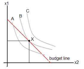
In the graph below, A, B and C are 3 ICs. We know from the properties of ICs that C represents the highest utility and A represents the least. Combination of x1 and x2 on C cannot be purchased by the consumer because they are beyond his budget. The points on A that lie within the budget set are affordable but not as preferred as bundles on B. So, the consumer will buy the bundle X. We get a unique, interior solution to the consumer's choice problem.


Graphically, the consumer will choose at bundle which lies at the point of tangency of the budget line and IC. So the optimal choice should be where the slope of the budget line is equal to the slope of the ICs, i.e., MRS = p1/p2.


budget-lines


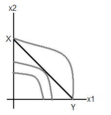
Violation of the axiom of strict convexity results in multiple or corner solutions as shown in the diagram below. X and Y are the optimal solutions because they lie on the highest IC on the budget line. At X, consumption of x1 is zero while at Y, consumption of x2 is

zero.

budget-line


Finding the optimal consumption bundle graphically can be tiresome and not effective if the consumer wishes to choose more than 2 commodities. It then becomes necessary to use mathematics. The consumer seeks to maximize U (x1, x2,....., xn) such that p1x1+p2x2+.....+pnxn ≤ m. This referred to as a constrained maximization problem.


The method to proceed is to define an auxiliary function:


L = U (x1, x2,....., xn) + λ (m - p1x1+p2x2+.....+pnxn).

λ, here is known as the Langrangian multiplier.

We then differentiate L with respect to each xi and equate them to zero. This gives us the first order conditions, i.e.,

δL/δx1= δU/δx1 - λp1 = 0 or δU/δx1 = λp1.


On repeating this step with the other xs and λ will generate (n+1) equations. Solving these equations simultaneously will give us the optimal xis which are amounts of commodities the consumer will demand. The xis will be expressed in terms of pis and m. If either the prices or the income of the consumer change then the amount of the commodities demanded will also change. The bundle of xis is known as the Marshallian demand bundle.


Substituting the solution values of xis in the objective utility function will produce the indirect utility function. This function gives the maximum utility that can be achieved by the consumer given the prices and his income.


If the mathematical approach seems difficult for you, take the help of Transtutors' online tutoring. In the tutoring sessions, professional tutors will clarify the mathematical procedure of maximization and then go on to interpret the results in economic terms.


Theory of Perfect competition


Perfect competition has the following characteristics:


  1. Large number of firms - There are a large number of firms in the market. Due to this each firm produces a very small fraction of the industry output. This is turn implies that a single firm cannot affect the market prices.
  2. Identical products - All the firms in market produce and sell an identical product. The consumers cannot differentiate between the product of one firm and that of another.
  3. Free entry and exit - New firms attracted by profit are free to enter the market while the existing ones suffering from losses are free to leave. Firms entering the market increase the supply of the good and reduce profit margins. Free exit reduces market supply and increases profit margins.
  4. Perfect information - All firms are fully informed about the prices and costs of their rival firms. Buyers have full information about prices and other relevant factors.


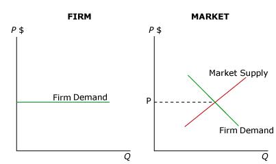
No firm can influence the market price by changing the quantity it supplies because of its relative small size in the market. The price is determined by the forces of total demand and total supply. Each firm takes the equilibrium price as given. The only variable that is under the control of a firm is its level of output. A firm decided on that output level that will maximise profits, given the prices. A single firm in the industry, therefore, is a price-taker and faces a horizontal demand curve at the equilibrium price. The industry, on the other hand, faces a demand curve that is downward-sloping. Together with industry supply curve, this determines the equilibrium price in the market.


perfact-comptition


How does the firm decide on its output level? On carrying out the profit maximization exercise, we derive the following condition for equilibrium: MR = MC. But since in perfect competition P = MR, the equilibrium is located at the point where P = MC. If price is greater than the MC then the firm should increase output further because it will add to profit. If price is less than the MC then the firm should not increase the output because the marginal unit produced at a loss.


In the long run, perfectly competitive firms earn zero profits. The free entry and exit in the markets is the reason behind this fact. When firms in the industry are making profits in the short run, new firms are attracted to enter the industry. This entry increases industry output and reduces the market price as well as the profits earned by each firm. This will continue as long as the existing firms keep earning positive profit. Entry will stop when profits have been reduced to zero.


Similarly, if the existing firms have been making losses in the short run, then these firms will exit the industry. This exit decreases industry output and causes an increase in the market price and reduction in losses incurred. As long as some firms are making losses, exit will continue. The process of exit stops when losses for all firms have been reduced to zero.


The only equilibrium in the long run is one in which all firms earn zero profits. Long-run equilibrium is depicted in the graph above. In long-run equilibrium, the perfectly competitive firm is producing efficiently at minimum average cost, at the intersection of line P* at point Q*. In the second graph showing the market scenario, the equilibrium price, P*, is found at the intersection of market supply and market demand.

General Equilibrium


General equilibrium studies the inter relationship between different markets. It is a situation where the plans of all the agents in all the markets are simultaneously realized. There are 2 types of general equilibrium analysis: Walrasian or Competitive general equilibrium and Non-Walrasian general equilibrium. In competitive general equilibrium, transactions take place only at equilibrium configurations. However, there are several situations where transactions may take place even without the plans of all agents being realized. Non-Walrasian general equilibrium deals with those cases.


One of the salient features of the Walrasian equilibrium is the Walras' law.  This law states that the sum of excess demand in all markets must be equal to zero. This implies that if there is positive excess demand in one market then there must be negative excess demand in some other market. Generally speaking, if (n-1) markets are cleared so is the remaining market.


General equilibrium analysis can be divided into 3 categories: (1) problem of optimal consumption, (2) problem of finding optimal production combination and (3) problem of optimal resources allocation. We will deal with the 2*2*2 model where it is assumed that the economy has 2 consumers, 2 goods and 2 factors of production.


Exchange Economy


Here we will concentrate on the exchange of goods among consumers, without taken production into account. This deals with the pricing and allocation issues confronted by a society. We begin by considering that each individual has an initial endowment of one or more of the commodity and is free to purchase or sell them at the market price depending on his utility function.


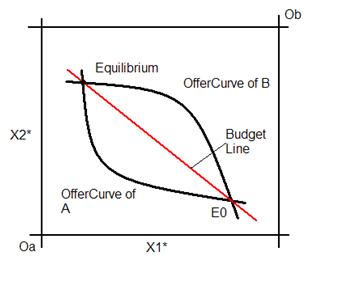
Let the 2 consumers be A and B. The total endowment of commodity 1 and commodity 2 are X1* and X2* respectively. Since we are dealing with 2 individuals simultaneously, we superimpose the commodity space of B on that of A to get a box diagram. The widtth of the box will be equal to X1* while its height will be X2*, if we measure commodity 1 on the horizontal axis and commodity 2 on the vertical axis. Once we start with a fixed endowment of the goods we have fixed dimensions of the box known as the Edgeworth box.


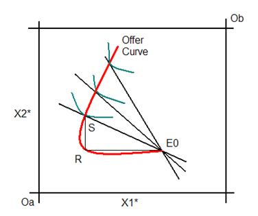
The diagram below illustrates an Edgeworth box. Oa and Ob are the origins for the respective individuals. The indifference curves away from the respective origins provide more utility. Any point on the box will give us an arbitrary endowment allocation, for example E0. The straight black lines through E0 with slope equal to the market price are the budget line for both individuals. A budget line separates the 2 feasible sets of A and B. It also depicts the exchange opportunities of A and B. The budget lines along with the indifference curves for the individuals gives us the optimal consumption choices of A and B. Suppose one such point, say S. At S, individual A has more of good one than he wants and therefore he will sell RE0 amount of the good. Similarly, he has less of good 2 and will demand RS amount of it. The locus of all the optimal consumption points of A is known as the offer curve. Any point on the offer curve of A, depicted in red, shows the price ruling in the market as well as the combination of buying and selling offers that A will make.


Exchange Economy


In the same manner, we can obtain the offer curve of B. On getting the 2 offer curves, you can notice the following properties of offer curves:


1.      Offer curves must pass through the endowment point because we can always show that there exists a price for which the endowment bundle is the most preferred bundle for both consumers.

2.      Offer curves lie in the better set of the endowment point.

3.      Offer curves are continuous if preferences are convex.

4.      Offer curves may be backward bending.

5.      Offer curve for A is the locus of the marginal rate of substitution of A while offer curve of B is the locus of marginal rate of substitution of B.


To know more about obtaining the offer curve as well its properties and their proofs, take the help of competent tutors at Transtutors. Depending on the level of knowledge you require, you can opt for online tutoring or assignment help.

The intersection of the 2 offer curves will give us the general equilibrium point. At this point, the plans of both A and B will be satisfied, i.e., the offers of both the individuals match. The equilibrium price will be the slope of the line joining E0 and the equilibrium point. Using the properties of offer curves, we can also claim that at the equilibrium point the marginal rate of substitution of both individuals will be the same and will be equal to the slope of the budget line or the market price.


general-equilibrium


For each endowment point we will get 2 sets of offer curves. There cannot be multiple equilibria because we cannot simultaneously start from 2 initial endowment points. At E0 the exchange takes place between the 2 consumers and the economy moves to the general equilibrium point. At this point there are no incentives for the individuals to trade because their plans have been realized. Since this new point lies in the better set for both individuals, it will be preferred by both.  However, it is essential that the markets are free and without any restrictions to trade.


We have seen what happens at the general equilibrium but we have to also learn to check for the existence, stability and uniqueness of the equilibrium. If the 2 offer curves do not intersect within the Edgeworth box then there is no feasible allocation which will be possible to achieve. Thus, the sufficient conditions for the existence of a Walrasian equilibrium are that both the offer curves must be continuous and at least one offer curve must be backward bending. Stability of the general equilibrium requires that the sum of excess demand elasticities in the two markets must exceed 1. Also, if the equilibrium in one market is unique, the other market should also posses a unique equilibrium.


thnx 4 sharing


CCI Pro

Leave a Reply

Your are not logged in . Please login to post replies

Click here to Login / Register